
[DAY 8] Pandas
Pandas
- 구조화된 데이터의 처리를 지원하는 Python 라이브러리
- Python계의 엑셀
- -panel data ➡ pandas
- 고성능 array 계산 라이브러리인 numpy와 통합하여, 강력한 “스프레드시트” 처리 기능을 제공
- 인덱싱, 연산용함수, 전처리함수 등을 제공함
- 데이터처리 및 통계분석을 위해 사용
- 이미지 처리를 위한 것이 아님
- tabular data에 최적화
- 행렬, 엑셀 시트 데이터
pandas 설치
1
2
3
4
5
  conda create -n 가상환경이름 python=3.8 # 가상환경생성
  activate 가상환경이름 # 가상환경실행
  conda install pandas # pandas 설치

  jupyter notebook # 주피터 실행하기
데이터 로딩
1
2
3
4
5
6
7
8
9
10
11
12
13
14
15
16
17
18
import pandas as pd  # 라이브러리 호출

# data_url = 'https://archive.ics.uci.edu/ml/machine-learning-databases/housing/housing.data' #Data URL
data_url = "./housing.data"  # Data URL

# csv 타입 데이터 로드, separate는 빈공간으로 지정하고, Column은 없음(없는 데이터를 불러왔다는 뜻)
df_data = pd.read_csv(data_url, sep="\s+", header=None)
"""
- data_url: web url 혹은 file
- sep: 데이터 분리기준
- "\s+": regex, s: single blank 의미, 띄어쓰기 많이를 기준으로 함

"""

df_data.head()  # 처음 다섯줄 출력
df_data.values  # array 타입으로 출력

type(df_data.values()) # numpy.ndarray
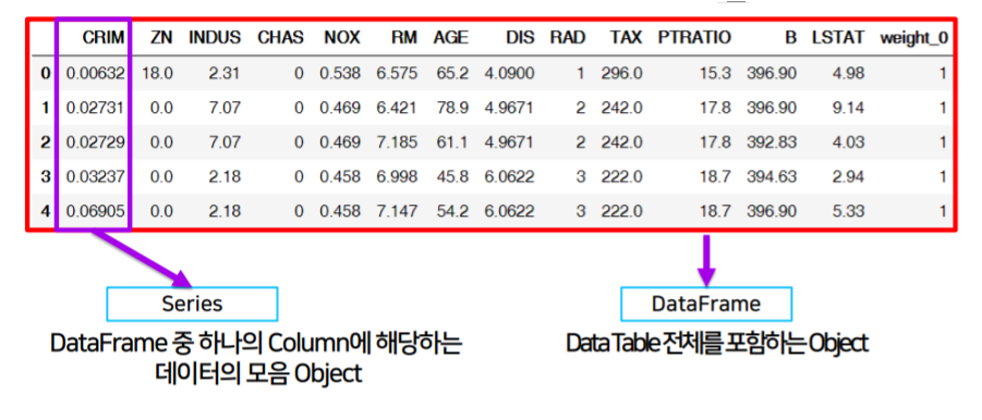
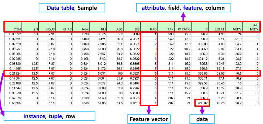
- Series: DataFrame 중 하나의 column에 해당하는 데이터의 모음 object
- DataFrame: Data Table 전체를 포함하는 Object
Series
df_data = pd.read_csv(data_url, sep="\s+", header=None): 기존 데이터를 불러와서 DataFrame 생성
1
2
3
4
5
6
7
8
9
10
11
12
13
14
15
16
17
18
19
20
21
22
23
24
25
26
27
28
29
30
31
32
33
34
35
36
37
38
39
40
41
42
43
44
45
46
47
48
49
50
51
52
53
54
55
56
57
58
59
60
61
62
63
64
65
66
67
68
69
70
71
72
73
74
75
76
77
78
79
80
81
82
83
84
85
86
87
88
89
90
91
92
93
94
95
96
97
98
99
100
101
102
103
104
105
106
107
108
109
110
111
112
from pandas import Series, DataFrame
import pandas as pd
import numpy as np

list_data = [1, 2, 3, 4, 5]
example_obj = Series(data=list_data) # column vector를 표현하는 object

"""
인덱스값(int) / Value
0    1
1    2
2    3
3    4
4    5
dtype: int64
"""

# 인덱스를 문자로 지정
list_data = [1, 2, 3, 4, 5]
list_name = ["a", "b", "c", "d", "e"]
example_obj = Series(data=list_data, index=list_name)

"""
인덱스값(문자) / Value
a    1
b    2
c    3
d    4
e    5
dtype: int64
"""

# dict 타입으로도 data와 인덱스를 설정할 수 있음
# key: 인덱스, value: 데이터
dict_data = {"a": 1, "b": 2, "c": 3, "d": 4, "e": 5}
example_obj = Series(dict_data, dtype=np.float32, name="example_data")

"""
a    1.0
b    2.0
c    3.0
d    4.0
e    5.0
Name: example_data, dtype: float32
"""

example_obj["a"] # 1.0

example_obj = example_obj.astype(float) # 타입변경
example_obj["a"] = 3.2 # 인덱스를 통해 값 변경

example_obj # 데이터 프레임
example_obj.index # 인덱스 리스트만 Index([,,,,], dtype='object?')
example_obj.values # 값 리스트만 array([,,,,], dtype=)

cond = example_obj > 2
example_obj[cond]
# example_obj[example_obj > 2]

example_obj * 2
"""
a     6.4
b     4.0
c     6.0
d     8.0
e    10.0
Name: example_data, dtype: float64
"""

np.exp(example_obj)  # np.abs , np.log
"""
a     24.532530
b      7.389056
c     20.085537
d     54.598150
e    148.413159
Name: example_data, dtype: float64
"""

"b" in example_obj # True False
example_obj.to_dict() # {'a': 3.2, 'b': 2.0, 'c': 3.0, 'd': 4.0, 'e': 5.0}

# Data에 대한 정보를 저장
example_obj.name = "number" # 칼럼이름
example_obj.index.name = "alphabet" # 인덱스 이름
"""
alphabet
a    3.2
b    2.0
c    3.0
d    4.0
e    5.0
Name: number, dtype: float64
"""

dict_data_1 = {"a": 1, "b": 2, "c": 3, "d": 4, "e": 5}
indexes = ["a", "b", "c", "d", "e", "f", "g", "h"]
series_obj_1 = Series(dict_data_1, index=indexes)
# "f", "g", "h"의 값이 없는 경우, index 값을 기준으로 series 생성되며
# 빈 value 자리에는 default=NaN 들어감
# ndarray는 index 기준으로 추가, 삭제!
"""
a    1.0
b    2.0
c    3.0
d    4.0
e    5.0
f    NaN
g    NaN
h    NaN
dtype: float64
"""
- Series는 사실상 numpy의 wrapper
- 데이터 프레임을 만들어냄
- 인덱스 값은 문자로도 지정 가능
- Series 는 numpy.ndarray의 subclass
- 어떤 타입의 데이터가 들어가든 상관없음
- 인덱스 레이블은 정렬되지 않음
복사 가능
1
2
3
4
5
6
7
# data type
float # default: float64
int # default: int 64
float32
int4
int8
int16
Dataframe
- Dataframe memory
- numpy array와 비슷
- 세로로 데이터 타입이 같고(한 column에 하나의 데이터 타입 가능)
- 가로로 데이터 타입이 다름(한 row에 여러 데이터 타입 가능)
- ➡ 각 column끼리는 같은 데이터 타입이고, row은 상관없음
- 가변적 크기: 컬럼 insert, delete 가능
- 하나의 데이터프레임 내의 값에 접근하기 위해서는 index, column 다 알아야함
- Series를 모아서 만든 DataTable ➡ 기본 2차원
- 실제로는 csv 가져와서 사용하는 경우가 대부분
NaN: Not a Number (값없음)
Dataframe 생성
1
2
3
4
5
6
7
8
9
10
11
12
13
14
15
16
17
18
19
20
21
22
23
24
25
26
27
28
29
30
31
32
33
34
35
from pandas import Series, DataFrame
import pandas as pd
import numpy as np

# Example from - https://chrisalbon.com/python/pandas_map_values_to_values.html
raw_data = {
    "first_name": ["Jason", "Molly", "Tina", "Jake", "Amy"],
    "last_name": ["Miller", "Jacobson", "Ali", "Milner", "Cooze"],
    "age": [42, 52, 36, 24, 73],
    "city": ["San Francisco", "Baltimore", "Miami", "Douglas", "Boston"],
}
df = pd.DataFrame(raw_data, columns=["first_name", "last_name", "age", "city"])
"""
column_name: data
key: column의 이름
보통은 csv를 불러옴
"""

df = DataFrame(raw_data, columns=["first_name", "last_name", "age", "city", "debt"])
# columns: 데이터 만드는 기준
# "debt" 추가되었으나, 값이 없으니 NaN표시
"""
    first_name  last_name   age   city            debt
0   Jason       Miller      42    San Francisco   NaN
1   Molly       Jacobson    52    Baltimore       NaN
2   Tina        Ali         36    Miami           NaN
3   Jake        Milner      24    Douglas         NaN
4   Amy         Cooze       73    Boston          NaN
"""

# column 선택 - series 추출
df.first_name # .: property type
df["first_name"] # dict 타입처럼 사용 가능, 결과는 같음

type(df["first_name"]) # pandas.core.series.Series # dtype: object
Dataframe indexing
loc: index location, 인덱스 이름iloc: index position, 인덱스 번호
1
2
3
4
5
6
7
8
9
10
11
12
13
14
15
16
17
18
19
20
21
22
23
24
25
26
27
28
29
30
df.loc[1] # 인덱스의 값이 들어감(문자도 가능) # 컬럼과 값이 나옴(row를 선택한 것일 것임)
df["age"].iloc[1:] # 숫자로 변환시켜 인덱스 접근가능

s = pd.Series(np.nan, index=[49, 48, 47, 46, 45, 1, 2, 3, 4, 5])
s.loc[:3] # 49, 48, 47, 46, 45, 1, 2, 3 해당하는 시리즈 추출
"""
49   NaN
48   NaN
47   NaN
46   NaN
45   NaN
1    NaN
2    NaN
3    NaN
dtype: float64
"""

s.iloc[:3] # [0]49, [1]48, [2]47
"""
49   NaN
48   NaN
47   NaN
dtype: float64
"""

df.loc[:, ["first_name", "last_name"]]
# index | first_name | last_name 으로 구성된 데이터 프레임 추출

# column에 새로운 값 할당 가능
df.debt = df.age > 40 # True/False value로 이루어진 debt 컬럼 생성
Dataframe Handling
1
2
3
4
5
6
7
8
9
10
11
12
13
14
15
16
17
18
19
20
21
22
23
24
25
26
27
28
29
values = Series(data=["M", "F", "F"], index=[0, 1, 3]) # 2, 4에는 NaN 들어감
"""
0    M
1    F
3    F
dtype: object
"""
df["sex"] = values # 이렇게 해줘야 df에 새로운 값 추가할 수 있음

df.head(3).T # Transpose # 일단 row 3개 뽑아서 행과 열을 바꾸어 보여줌
"""
            0       1         2
first_name  Jason   Molly     Tina
last_name   Miller  Jacobson  Ali
age         42      52        36
city        LA      Baltimore Miami
debt        True    True      False
sex         M       F         NaN
"""

# csv 변환
df.to_csv()
"""
index=false 인자 주면 인덱스 값 제거
df.index -> RangeIndex(start=0, stop=5, step=1)
"""

# column 삭제(메모리 주소 자체를 삭제)
del df["debt"]
Selection & Drop
- Selection: 선택, 데이터 쿼리, column 이름을 통해 가져오기가 제일 쉬움
- Drop: 삭제, 드롭 이후(col 삭제 이후) 데이터 프레임을 보여주고, 이는 저장되지 않음(only 리턴)
1
2
3
4
5
6
7
8
9
10
11
12
13
14
15
16
17
18
19
20
21
22
23
24
25
26
27
28
29
30
31
32
33
34
35
36
37
38
39
40
41
42
43
44
45
46
47
48
49
50
51
52
53
54
55
56
57
58
59
60
61
62
63
64
65
66
67
68
69
70
71
72
73
74
75
76
77
78
79
80
81
82
83
84
85
86
87
88
89
90
91
92
93
94
95
96
97
98
99
100
101
102
103
104
105
106
107
108
109
110
111
112
113
114
115
116
117
pop = {"a":{0: "choco", 1: "coffee"}, "b": {}}
DataFrame(pop)
# 이때 "a", "b"는 column
# dict의 key = index

df.drop("debt", axis=1) # axis=1 : column 기준 삭제
# -> 저장되지 않음

# -------------------------------------------------- Selection with names
# 1개의 column 선택
account_serires = df["account"] # list가 아닌 column, series 임
account_serires[:3] # 시리즈 데이터
# df["account"].head(3) #와 같음

# 1개 이상의 column 선택
# 데이터 프레임의 형태: [[]]
df[["account", "street", "state"]].head(3)
# ["account", "street", "state"] 리스트 형태로 col의 이름을 넣어서 가져오기 가능

# ----------------------------------------------- Selection with index number
# column 이름 없이 사용하는 index number는 row기준 표시
df[:3]
# 만약 a, b, c 라면 이렇게 안뽑힘
# 약간 일관성 없는거같은,,,
"""
숫자 -> 인덱스 인식 -> row -> 출력 (DF형식)
  account name street city state postal-code Jan Feb Mar
0 211829 Kerluke, Koepp and Hilpert 34456 Sean Highway New Jaycob Texas 28752 10000 62000 35000
1 320563 Walter-Trantow 1311 Alvis Tunnel Port Khadijah NorthCarolina 38365 95000 45000 35000
2 648336 Bashirian, Kunde and Price 62184 Schamberger Underpass Apt. 231 New Lilianland Iowa 76517 91000 120000 35000
"""

# column 이름과 함께 row index 사용시, 해당 column만 출력
df["name"][:3]
"""
0    Kerluke, Koepp and Hilpert
1                Walter-Trantow
2    Bashirian, Kunde and Price
Name: name, dtype: object
"""

# 한개 이상의 index
account_serires[[1, 5, 5, 2]] # 리스트 형태로 인덱스 넣을 수 있음
""
1    320563
5    132971
5    132971
2    648336
Name: account, dtype: int64
""

# fancy index 처럼 사용 가능
account_serires[list(range(0,5,2))] # 범위지정 list 가능 # 0, 2, 4, ..., 14
account_serires[account_serires < 250000] # boolean index 가능 (True인 경우에만 가져와서 출력해줌)

# ------------------------------------------------------------ index 변경
df.index = df["account"]
del df["account"] # 해당하는 컬럼 삭제
df.head()

# ----------------------------------------------- basic, loc, iloc selection
# basic
df[["name", "street"]][:2] # column과 index number
"""
          name                          street
account
211829    Kerluke, Koepp and Hilpert    34456 Sean Highway
320563    Walter-Trantow                1311 Alvis Tunnel
"""

# loc[col, index_name]
df.loc[[211829, 320563], ["name", "street"]]
# [211829, 320563] : row의 인덱스 번호
#   -> 분명한 인덱스로 넣어야함 # [:2]불가 # :32563 가능
# ["name", "street"] : col의 이름

# iloc[col_num, index_num]
df.iloc[:10, :3]
# col: 앞에서 10개
# row: 앞에서 2개

# ---------------------------------------------------------------- reindex
# 인덱스 재설정
df.index = list(range(0, 15))
df.reset_index(inplace=True)
"""
reset_index(): 인덱스 추가
drop=True: 기존 인덱스 제거
inplace=True: DF 자체가 변화

default) 제거없이 오직 추가만하며, 원본을 변경하지 않고 오직 리턴함
"""

# ---------------------------------------------------------------- drop
df.drop(1)

df.drop(1, inplace=True) # inplace=True 해야 값이 변경
df.drop([0, 1, 2, 3]) # 한개 이상의 index number로 drop
# 여러 row를 한번에 제거 가능

matrix = df.values
matrix[:3]
matrix[:, -3:]

matrix[:, -3:].sum(axis=1)

df.drop("city", axis=1) # axis 지정으로 축을 기준으로 drop ➡ column중에 "city"
df.drop(["city", "state"], axis=1) # 컬럼제거
# | : axis=0
# ㅡ : axis=1

"""
inplace=False: (default) 값의 변화 없음
inplace=True: 원본데이터 변경
"""

df.as_matrix()
- 보통 column:str, index:num 사용
!conda install --y xlrd엑셀 핸들링모델
Dataframe Operations
Series Operation
- 인덱스 중복 허용
- with numpy, Series, DF에서 똑같은 연산 일어남
1
2
3
4
5
6
7
8
9
10
11
12
13
14
15
16
17
18
19
20
21
22
23
24
25
26
27
28
s1 = Series(range(1, 6), index=list("abced"))
s2 = Series(range(5, 11), index=list("bcedef"))
"""
s1        s2
------------------
a    1    b     5
b    2    c     6
c    3    e     7 ✔
e    4 ✔  d     8
d    5    e     9 ✔
          f    10
dtype: int64
"""

s1 + s2
s1.add(s2) # 두개는 결과가 같음
"""
인덱스 기준으로 연산을 수행
겹치는 인덱스(둘 중 하나라도 값이 없는 경우)가 없을 경우, NaN을 가지는 데이터 생성
a     NaN
b     7.0
c     9.0
d    13.0
e    11.0
e    13.0
f     NaN
dtype: float64
"""
Dataframe Operation
- df는 column과 index를 모두 고려
1
2
3
4
5
6
7
8
9
10
11
12
13
14
15
16
17
18
19
20
21
22
23
24
25
26
27
28
29
30
31
32
33
34
35
36
37
38
39
40
41
42
43
44
45
46
47
48
# col, index 함께 확인
df1 = DataFrame(np.arange(9).reshape(3, 3), columns=list("abc"))
"""
a	b	c
0	0	1	2
1	3	4	5
2	6	7	8
"""
df2 = DataFrame(np.arange(16).reshape(4, 4), columns=list("abcd"))
"""
	a	b	c	d
0	0	1	2	3
1	4	5	6	7
2	8	9	10	11
3	12	13	14	15
"""

df1 + df2
"""
둘 중에 하나라도 값이 없으면 NaN으로 채움
	a	b	c	d
0	0.0	2.0	4.0	NaN
1	7.0	9.0	11.0	NaN
2	14.0	16.0	18.0	NaN
3	NaN	NaN	NaN	NaN
"""

df1.add(df2, fill_value=0)
"""
둘 중 하나라도 없으면 데이터가 NaN으로 만들어지는 것을 보완하여,
NaN값의 경우를 0으로 만들어서 연산할 수 있게 만듦
	a	b	c	d
0	0.0	2.0	4.0	3.0
1	7.0	9.0	11.0	7.0
2	14.0	16.0	18.0	11.0
3	12.0	13.0	14.0	15.0
"""

df1.mul(df2, fill_value=1)
"""
a	b	c	d
0	0.0	1.0	4.0	3.0
1	12.0	20.0	30.0	7.0
2	48.0	63.0	80.0	11.0
3	12.0	13.0	14.0	15.0
"""

# operation types: add, sub, div, mul
Series + Dataframe
- Dataframe과 Series 연산시, 브로드캐스팅을 위해 인덱스 위치 혹은 axis 정해주어야함(기준값 필요)
1
2
3
4
5
6
7
8
9
10
11
12
13
14
15
16
17
18
19
20
21
22
23
24
25
26
27
28
29
30
31
32
33
34
35
36
37
38
39
40
41
42
43
44
45
46
47
48
49
50
51
df = DataFrame(np.arange(16).reshape(4, 4), columns=list("abcd"))
"""
a	b	c	d
0	0	1	2	3
1	4	5	6	7
2	8	9	10	11
3	12	13	14	15
"""

s = Series(np.arange(10, 14), index=list("abcd"))
"""
인덱스가 어딘지 정해준 경우, 일반 연산시 방향을 알 수 있으므로 Broadcasting
a    10
b    11
c    12
d    13
dtype: int32
"""

df + s
"""
s의 인덱스가 어딘지 알기 때문에 broadcasting 가능
	a	b	c	d
0	10	12	14	16
1	14	16	18	20
2	18	20	22	24
3	22	24	26	28
"""

s2 = Series(np.arange(10, 14))
df + s2
"""
인덱스가 무엇인지 알려주지 않음 -> NaN값!
	a	b	c	d	0	1	2	3
0	NaN	NaN	NaN	NaN	NaN	NaN	NaN	NaN
1	NaN	NaN	NaN	NaN	NaN	NaN	NaN	NaN
2	NaN	NaN	NaN	NaN	NaN	NaN	NaN	NaN
3	NaN	NaN	NaN	NaN	NaN	NaN	NaN	NaN
"""

df.add(s2, axis=0)
"""
축을 정해주는 경우, 축(axis=0)을 기준으로 row broadcasting 실행
a	b	c	d
0	10	11	12	13 (+10)
1	15	16	17	18 (+11)
2	20	21	22	23 (+12)
3	25	26	27	28 (+13)

원본 변경 이뤄지는가?
"""
lambda, map, apply
map of series
- pandas의 series type의 데이터에도 map 함수 사용 가능
- function 대신 dict, sequence형 자료등으로 대체 가능
1
2
3
4
5
6
7
8
9
10
11
12
13
14
15
16
17
18
19
20
21
22
23
24
25
26
27
28
29
30
31
32
33
34
35
36
37
38
39
40
41
42
43
44
45
46
47
48
49
50
51
52
53
54
55
56
57
58
59
60
61
62
63
64
65
66
67
68
69
70
71
72
import pandas as pd
import numpy as np
from pandas import Series

# ------------------------------------------- lambda
f = lambda x, y: x + y
f(1, 4)

def f(x, y):
    return x + y

f = lambda x: x ** 2
f(3)

f = lambda x: x + 5
f(3)

(lambda x: x + 1)(5)

# ----------------------------------------------- map
ex = [1, 2, 3, 4, 5]
f = lambda x: x ** 2
list(map(f, ex))

f = lambda x, y: x + y
list(map(f, ex, ex))

list(map(lambda x: x + 5, ex))
# python 3에는 list를 꼭 붙여줘야함

s1 = Series(np.arange(10))
s1. head(5)

def f(X):
  return x+5
# f = lambda x: x**2
s1.map(f)
# 출력은 하지만 원본의 값은 변하지 않음

z = {1,=: "A", 2: "B", 3: "C"}
s1.map(z) => 값이 변하고 남은 자리에는 NaN 들어감

s2 = Series(np.arange(10, 30))’
# 인덱스: 0~19
# 값: 10~29

s1.map(s2)
# 같은 인덱스 값만 맵핑 # s1의 갯수가 10개라면 s2의 값 10개만 가져와서 s1을 바꿈

# ----------------------------------------- 예제
# !wget https://raw.githubusercontent.com/rstudio/Intro/master/data/wages.csv
df = pd.read_csv("./data/wages.csv")
df.head()

df.sex.unique()
array(['male', 'female'], dtype=object)

def change_sex(x):
  return 0 if x=="male" else 1
df.sex.map(change_sex)
# 원본 df.sex는 전혀 변화없음

df["code"] = df.sex.map({"male": 0, "female": 1}) # 성별 str -> 성별 code
# 산출된 값을 할당해줌
# dict type 활용

df["code"] = df.sex.map({"male": 0, "female": 1}, inplace=True)
# 이렇게해야 변경됨

df.drop("code", axis=1, inplace =True)
# 완전히 삭제
# inplace 안넣으려면 del 쓰면됨
1
2
3
4
5
6
7
8
9
10
11
12
13
14
15
16
17
18
19
20
21
22
23
24
25
26
27
28
29
30
31
32
33
34
35
# -------------------------------------- map & replcae
s1 = Series(np.arange(10))
s1.head(5)

s1.map(lambda x: x**2).head(5)
# 각 원소의 값이 제곱됨

# 모든 원소값에 대해 함수 적용(1, 2, 3)
# 1번
def f(x):
  return x+5
s1.map(f)

# 2번 # dict type으로 데이터 교체, 없는 값은 NaN
z = {1: 'A', 2: 'B', 3:'C'}
s1.map(z).head(5)
# 예를들어 value가 1이면 value값이 'A'로 바뀌어 들어감
"""
0    NaN
1      A
2      B
3      C
4    NaN
5    NaN
6    NaN
7    NaN
8    NaN
9    NaN
dtype: object
"""

# 3번 # 같은 위치의 데이터를 s2로 전환(인덱스 기준 맵핑)
s2 = Series(np.arange(10, 30))
s1.map(s2)
# dict와 series 둘다 가능
replace function
- 데이터 자체를 변화시킴
- map func 사용
- dict type 적용
df.col.replace([target_list], [conversion_list], inplace=True)inplace=True: 데이터 변환결과를 적용
1
2
3
df.sex.replace({"male": 0, "female": 1})
df.sex.replace(["male", "female"], [0, 1], inplace=True)
del df["sex_code"]
apply for dataframe
- map과 달리, series 전체(column)에 해당함수를 적용
- 입력값이 series 데이터로 입력받아 handling 가능
- DF에 적용하는 경우, 모든 series(컬럼)에 적용됨
- 각 column별로 결과값을 반환
- 내장 연산 함수를 사용할 때에도 똑같은 효과를 거둘 수 있음
- mean, std등 사용가능
df_info.sum()=df_info.apply(sum)
스칼라(scalar)값 이외에 series값의 반환도 가능(각 시리즈마다 적용가능 - 통계치 쓸 때 사용됨)
apply(): series에 적용applymap(): 모든 값에 적용
1
2
3
4
5
6
7
8
9
10
11
12
13
14
15
16
17
18
19
20
21
22
23
24
25
26
27
28
29
30
31
32
33
34
35
36
37
38
39
40
41
42
43
44
45
46
47
48
49
50
51
52
53
54
55
56
57
58
59
60
61
62
63
64
65
66
67
df = pd.read_csv("wages.csv")

df_info = df[["earn", "height", "age"]]
df_info.head()
"""
  earn	height	sex	race	ed	age
0	79571.299011	73.89	male	white	16	49
1	96396.988643	66.23	female	white	16	62
2	48710.666947	63.77	female	white	16	33
3	80478.096153	63.22	female	other	16	95
4	82089.345498	63.08	female	white	17	43
"""

# 아래 셋의 결과는 같음
f = lambda x: np.mean(x) # 1
df_info.apply(f)
df_info.apply(np.mean) # 2
df_info.mean() # 3
"""
earn      32446.292622
height       66.592640
age          45.328499
dtype: float64
"""

# 스칼라(scalar)값 이외에 series값의 반환도 가능(각 시리즈마다 적용가능
def f(x):
    return Series(
        [x.min(), x.max(), x.mean(), sum(x.isnull())],
        index=["min", "max", "mean", "null"],
    )
df_info.apply(f)
"""
earn	height	age
min	-98.580489	57.34000	22.000000
max	317949.127955	77.21000	95.000000
mean	32446.292622	66.59264	45.328499
null	0.000000	0.00000	0.000000
"""

f = lambda x: x // 2
df_info.applymap(f).head(5)
"""
	earn	height	age
0	39785.0	36.0	24
1	48198.0	33.0	31
2	24355.0	31.0	16
3	40239.0	31.0	47
4	41044.0	31.0	21
"""

f = lambda x: x ** 2
df_info["earn"].apply(f)
"""
0       6.331592e+09
1       9.292379e+09
2       2.372729e+09
3       6.476724e+09
4       6.738661e+09
            ...
1374    9.104329e+08
1375    6.176974e+08
1376    1.879825e+08
1377    9.106124e+09
1378    9.168947e+07
Name: earn, Length: 1379, dtype: float64
"""
Pandas built-in Functions
- pandas가 이미 가지고 있는 함수
describe(): numeric type(숫자형) 데이터의 요약정보를 보여줌(int, float, bool only)unique(): series data의 유일한 값을 list로 반환sum(): 기본적인 column 또는 row값의 연산을 지원(sub, mean, max, count, median, mad, var 등)isnull(): column 또는 row 값의 NaN(null)값의 인덱스를 반환함sort_values(): column값을 기준으로 데이터를 sorting.corr()&.cov()&.corrwith(): 상관계수와 공분산을 구하는 함수
1
2
3
4
5
6
7
8
9
10
11
12
13
14
15
16
17
18
19
20
21
22
23
24
25
26
27
28
29
30
31
32
33
34
35
36
37
38
39
40
41
42
43
44
45
46
47
48
49
50
51
52
53
54
55
56
57
58
59
60
61
62
63
64
65
66
67
68
69
70
71
72
73
74
75
76
77
78
79
80
81
82
83
84
85
86
87
88
89
90
91
92
93
94
95
96
97
98
99
100
101
102
103
104
105
106
107
108
109
110
111
112
113
114
115
116
117
118
119
120
121
122
123
124
125
126
127
128
129
130
131
132
133
134
135
136
137
138
139
140
141
142
143
144
145
146
147
148
149
150
151
152
153
df = pd.read_csv("data/wages.csv")
df.head(2).T
"""
      0    	1
earn	79571.3	96397
height	73.89	66.23
sex	male	female
race	white	white
ed	16	16
age	49	62
"""

# ----------------------------------------------------------- describe
df.describe()
"""
      earn	height	ed	age
count	1379.000000	1379.000000	1379.000000	1379.000000
mean	32446.292622	66.592640	13.354605	45.328499
std	31257.070006	3.818108	2.438741	15.789715
min	-98.580489	57.340000	3.000000	22.000000
25%	10538.790721	63.720000	12.000000	33.000000
50%	26877.870178	66.050000	13.000000	42.000000
75%	44506.215336	69.315000	15.000000	55.000000
max	317949.127955	77.210000	18.000000	95.000000
"""

# ----------------------------------------------------------- unique
# df.types: 각 컬럼별로 타입을 보여줌

key = df.race.unique() # 유일한 인족의 값
# array(['white', 'other', 'hispanic', 'black'], dtype=object)

# 라벨링 코딩
key = df.race.unique()
value = range(len(df.race.unique()))
df["race"].replace(to_replace=key, value=value)

dict(enumerate(sorted(df["race"].unique()))) # 숫자와 묶어줌
# {0: 'white', 1: 'other', 2: 'hispanic', 3: 'black'}

np.array([dict(enumerate(df["race"].unique()))]) # dict type으로 index
# array({0: 'white', 1: 'other', 2: 'hispanic', 3: 'black'}, dtype=object)

# label index값과 label값 각각 추출
value = list(map(int, np.array(list(enumerate(df["race"].unique())))[:, 0].tolist()))
key = np.array(list(enumerate(df["race"].unique())), dtype=str)[:, 1].tolist()

# -------------------------------------
# label str ➡ index 값으로 변환
df["race"].replace(to_replace=key, value=value, inplace=True)

# 성별에 대해서도 동일하게 적용
value = list(map(int, np.array(list(enumerate(df["sex"].unique())))[:, 0].tolist()))
key = np.array(list(enumerate(df["sex"].unique())), dtype=str)[:, 1].tolist()
# ([0, 1], ['male', 'female'])

df["sex"].replace(to_replace=key, value=value, inplace=True)
# "sex"와 "race" column의 index labelling

# ----------------------------------------------------------- sum
numueric_cols = ["earn", "height", "ed", "age"]
df[numueric_cols].sum(axis=1)

df.sum(axis=0) # column 별
"""
earn ~~~
height ~~~
"""
df.sum(axis=1) # row 별
"""
0 ~~~
1 ~~~
"""

# -------------------------------------------------------- isnull
df.isnull() # True/False
df.isnull().sum() # 빈 것의 개수 세기(null인 값의 합)
df.isnull().sum() / len(df) # null인 값의 비율

pd.options.display.max_rows = 100

# ------------------------------------------------------ sort_values
df.sort_values(["age", "earn"], ascending=True)
# 오름차순으로, column값 기준으로 데이터 sort
# 인덱스 값이 섞여서 나옴
"""
    earn	height	sex	race	ed	age
1038	-56.321979	67.81	male	hispanic	10	22
800	-27.876819	72.29	male	white	12	22
963	-25.655260	68.90	male	white	12	22
1105	988.565070	64.71	female	white	12	22
801	1000.221504	64.09	female	white	12	22
"""

df.sort_values("age", ascending=False).head(10)
"""
    earn	height	sex	race	ed	age
3	80478.096153	63.22	female	other	16	95
331	39169.750135	64.79	female	white	12	95
809	42963.362005	72.94	male	white	12	95
102	39751.194030	67.14	male	white	12	93
993	32809.632677	59.61	female	other	16	92
1017	8942.806716	62.97	female	white	10	91
1192	39757.947210	64.79	male	white	16	90
952	8162.682672	58.09	female	white	5	89
827	55712.348432	70.13	male	white	9	88
1068	10861.092284	64.03	female	white	13	87
"""

# -------------------------------------------------- cov, corr, corrwith
df.age.corr(df.earn) # df.age ↔ df.earn 두 컬럼 사이의 상관계수 # 0.07400349177836055

df.age[(df.age < 45) & (df.age > 15)].corr(df.earn) # 0.31411788725189044

df.age.cov(df.earn) # 공분산 # 36523.6992104089

df["sex_code"] = df["sex"].replace({"male": 1, "female": 0})

df.corr() # 상관계수 # 모든 상관관계를 한번에 보여줌
"""
	    earn	height	ed	age	sex_code
earn	1.000000	0.291600	0.350374	0.074003	0.337328
height	0.291600	1.000000	0.114047	-0.133727	0.703672
ed	0.350374	0.114047	1.000000	-0.129802	0.061747
age	0.074003	-0.133727	-0.129802	1.000000	-0.070036
sex_code	0.337328	0.703672	0.061747	-0.070036	1.000000
"""

df.corrwith(df.earn)

df.sex.value_counts(sort=True)

# ---------------------------------------------------------- Additional Info

# 여러 col이 다를때, list 형태로 저장시키고
list = [ , ,  ,]
df[list].sum(axis=1) # 가능 => 이게 selection
# 그러나 만약 string인 경우에는 concat되므로 값이 이상해짐
# numeric 데이터에만 사용할 것!

pd.options.display.max_rows = 100
# 최대 출력수 지정(생략하지 않고 보여줌)

df.age[df.age < 45].corr(df.earn) # [bool] 괄호 안의 조건이 참인 경우의 값만 가져옴

df["sx"] = df["sx"].replace({"male":1, "female":0})
# string으로 처리하기 힘들기 떄문에 0과 1로 바꾸어줌 -> 라벨링 코딩

# 글자의 수
df.sx.value_counts(sort=True)
# object type의 경우,
# female---
# male---